1. GoogLeNet이란?
GoogLeNet이란 2014년 Google에서 개발한 CNN모델로 ILSVRC 2014(ImageNet Large Scale Visual Recognition Challenge)에서 우승을 차지하였습니다.
주어진 HW자원을 최대한 효율적으로 이용하면서 학습은 극대화할 수 있는 깊고 넓은 신경망입니다.
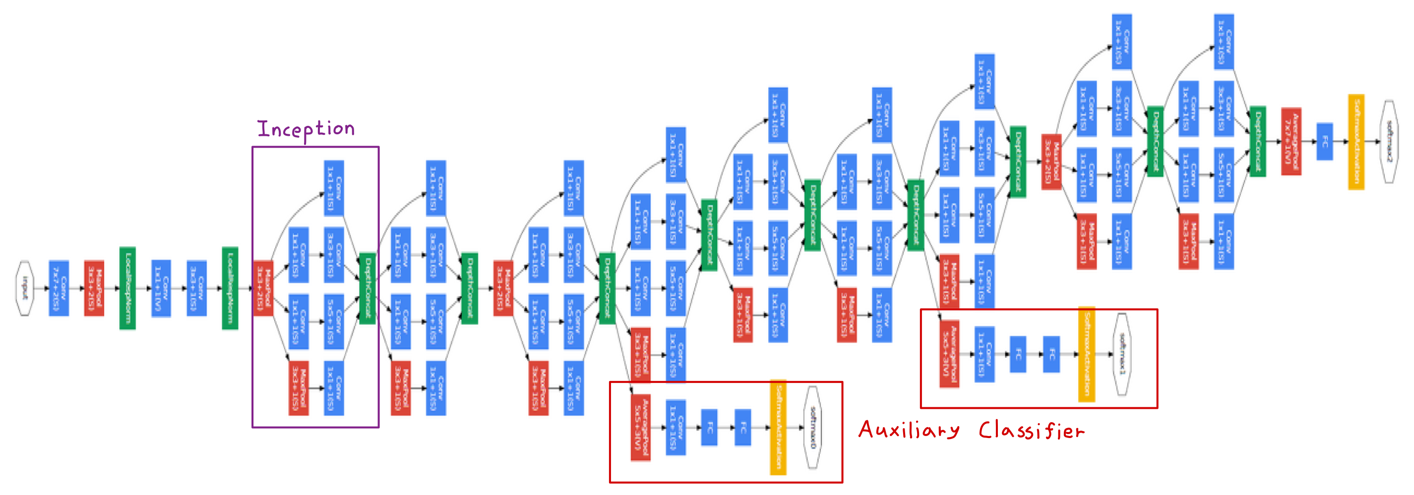
깊고 넓은 신경망을 위해 Inception Module을 추가하였습니다. 이를 통해 네트워크의 Depth와 Width를 늘리면서도 Computational Efficiency를 확보하였습니다.
GoogLeNet 특징
- Inception Module : 여러 크기의 Convolution Filter(1x1, 3x3, 5x5)를 동시에 적용하여 네트워크가 다양한 크기의 패턴을 학습, 더 깊고 더 넓은 네트워크 구조를 효율적으로 처리 가능
- 1 x 1 Convolution : 1x1 Convolution Filter를 사용하여 차원의 수를 줄임. 이를 통해 계산량을 줄이면서도 중요한 정보를 보존할 수 있다.
- Model의 Depth : 22개의 Layer로 구성, 매우 깊은 네트워크 구조를 가지고 있지만 복잡성을 줄이기 위해 상대적으로 적은 수의 파라미터 사용
- 성능과 효율성 : 다른 CNN 모델보다 더 적은 파라미터를 사용하면서도 우수한 성능
2. GoogLeNet 구조
GoogLeNet의 구조는 Inception Module을 중심으로 설계되었습니다. 따라서 먼저 Inception Module에 대해 알아보겠습니다.
2-1) Inception Module
Feafure를 효율적으로 추출하기 위해 여러 크기의 Convolution Filter(1x1, 3x3, 5x5)를 병렬적으로 적용하여, 네트워크기가 다양한 크기의 특징을 동시에 학습할 수 있도록 합니다.
즉, Image의 다양한 영역을 볼 수 있도록 서로 다른 크기의 Filter를 사용하여 Ensemble하는 효과를 가져와 Parameter를 효율적으로 사용할 수 있게 됩니다.

1 x 1 Filter
공간적인 크기를 변경하지 않으면서, 각 채널에 대해 연산 수행을 수행합니다.
이를 통해 Input Data를 더 작은 차원으로 줄이거나, 중요한 Feature만을 추출할 수 있습니다.
3 x 3 Filter
주변 Pixel들과의 관계를 포착하여 패턴을 학습니다.
중간 크기의 특징을 잡아내는 데 유용하며, 일반적으로 Image에서 중요한 세부 정보를 추출하는데 많이 사용됩니다.
5 x 5 Filter
큰 공간적 범위에서 정보를 처리할 수 있습니다. 따라서 큰 패턴이나 긴 거리의 관계를 학습하는데 유리합니다.\
이처럼 다양한 크기의 Filter를 동시에 적용하여, 여러 크기의 패턴을 동시에 학습할 수 있게 됩니다.
이렇게 여러 크기의 Filter를 동시에 사용하면, Network가 다양한 크기의 특징을 동시에 추출할 수 있으며, 다양한 패턴을 효과적으로 추출할 수 있습니다.
위의 Naive version은 Inception Module 내에서 각 필터를 그대로 적용하고, 이를 직접적으로 이어붙여 사용합니다. 하지만 이 방식에서는 각 Filter의 출력이 채널 차원을 늘려서 합쳐집니다. 따라서 Filter의 크기와 채널 수가 커질수록 연산량이 증가하는 문제가 발생할 수 있습니다.
따라서, 아래와 같이 Inception Module에 Dimension Reduction을 적용할 수 있습니다.

Inception Module에 1 x 1 Convolution Filter를 먼저 적용하여 Channel수를 줄인 후에, 3 x 3, 5 x 5 Filter를 사용합니다.
앞서 설명했듯이 1 x 1 Filter는 주로 차원 축소역할을 하기 때문에 연산량을 크게 줄일 수 있습니다.
즉, 1 x 1 Filter는 Input Data의 채널 수를 줄여서, 3 x 3과 5 x 5 Filter가 적용할 데이터의 크기를 줄여 전체 연산량이 감소하게 됩니다.
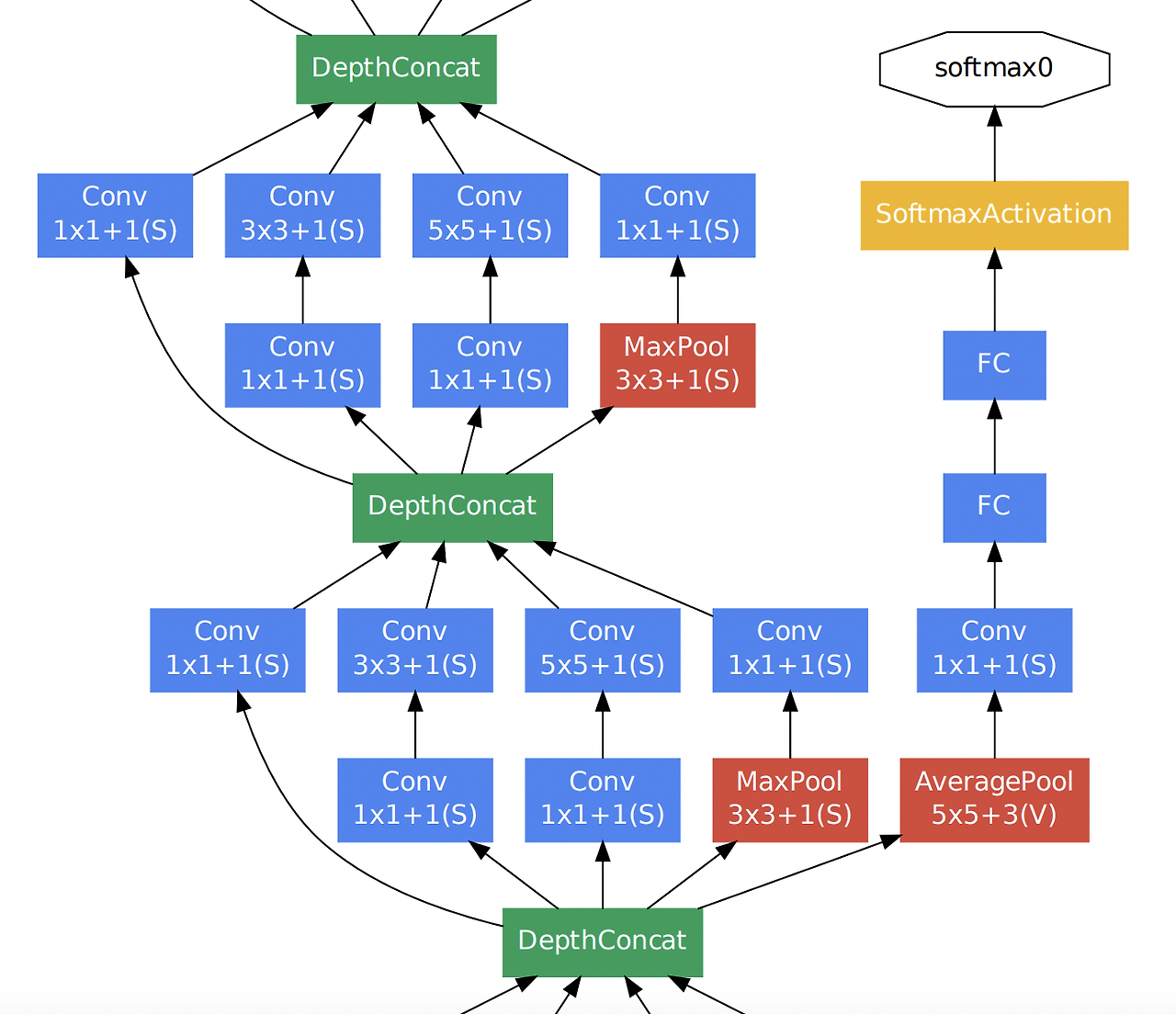
2-2) Auxiliary Classifier
GoogLeNet은 Auxiliary Classifier라는 중간 분류기를 도입하여, Network의 학습을 돕습니다.
중간 단계에서 예측을 수행하여 Backpropagation 과정에서 신경망의 학습을 원할하게 하고 Overffitng을 방지합니다.
조금 더 자세하게 설명하면, Network 깊어지면서 Loss에 대한 역전파 과정에서 발생할 수 있는 Gradient Vanishing 문제를 해결하기 위해 도입되었습니다.
이렇게 함으로써 중간에 있는 Inception Module들도 적절한 가중치 업데이트를 받을 수 있게 됩니다.
하지만 Inception Module의 버전이 발전함에 따라 역전파를 통해 학습이 적절하게 이루어 졌지만, 최종 Classifier에서는 학습이 잘 이루어지지 않는 문제가 생겨 Inception v4에서는 완전히 제외되었습니다.
2-3) Global Average Pooling(GAP)
GoogLeNet에서는 전통적인 FC Layer 대신 Global Average Pooling을 사용합니다.
이는 마지막 FC Layer에서 각 Channel의 평균값을 계산하여 모델의 파라미터 수를 줄이고 Overfitting을 방지하는 역할을 합니다.
그 이유는 Convolution Layer 연산의 결과들로 만들어진 Feature Map을 FC Layer에 넣고 최종적으로 분류하는 과정에서 공간 정보가 손실되기 때문입니다.
GAP는 채널별 Featue Map 평균을 구해 직접 Softmax Layer의 입력으로 사용하여 공간 정보가 손실되지 않을 뿐만 아니라 FC Layer에 의해 파라미터를 최적화하는 과정이 없기 때문에 효율적입니다.

2-4) GoogLeNet 전체 구조
3. GoogLeNet Pytorch 구현
1) 필요한 라이브러리 호출
import torch
import torch.nn as nn
import torch.optim as optim
import torch.nn.functional as F
import torchvision
import torchvision.transforms as transforms
from torch.utils.data import DataLoader
import torchvision.datasets as datasets

device = torch.device("cuda" if torch.cuda.is_available() else "cpu")
2) Inception Module 구현
Inception Module에 Dimension Reduction이 적용된 버전입니다.
3 x 3, 5 x 5 Filter를 적용하기 전 1 x 1 Filter를 적용하여 차원을 축소합니다.
그 후, 각 Branch를 Concat합니다.
class Inception(nn.Module):
    def __init__(self, in_channels, out1x1, out3x3_reduce, out3x3, out5x5_reduce, out5x5, outpool):
        super(Inception, self).__init__()

        # 1 x 1 Convolution
        self.conv1x1 = nn.Conv2d(in_channels, out1x1, kernel_size=1, stride=1)

        # Inception Module에 Dimension Reduction 적용
        # conv3x3_reduce : 3x3 Convolution Layer 전 1x1 Filter 적용
        self.conv3x3_reduce = nn.Conv2d(in_channels, out3x3_reduce, kernel_size=1, stride=1)
        self.conv3x3 = nn.Conv2d(out3x3_reduce, out3x3, kernel_size=3, stride=1, padding=1)

        self.conv5x5_reduce = nn.Conv2d(in_channels, out5x5_reduce, kernel_size=1, stride=1)
        self.conv5x5 = nn.Conv2d(out5x5_reduce, out5x5, kernel_size=5, stride=1, padding=2)

        self.maxpool = nn.MaxPool2d(kernel_size=3, stride=1, padding=1)
        self.convpool = nn.Conv2d(in_channels, outpool, kernel_size=1, stride=1)

    def forward(self, x):
        # 1 x 1 Convolution Path
        path1 = F.relu(self.conv1x1(x))

        # 3 x 3 Convolution Path
        path2 = F.relu(self.conv3x3_reduce(x))
        path2 = F.relu(self.conv3x3(path2))

        # 5 x 5 Convolution Path
        path3 = F.relu(self.conv5x5_reduce(x))
        path3 = F.relu(self.conv5x5(path3))

        # Max Pooling Path
        path4 = self.maxpool(x)
        path4 = F.relu(self.convpool(path4))

        return torch.cat([path1, path2, path3, path4], dim=1)
3) Auxiliary Classifier 구현
Auxiliary Classifier는 보통 Inception 3 Layer와 연결되어 사용합니다.
class AuxiliaryClassifier(nn.Module):
    def __init__(self, in_channels, num_classes):
        super(AuxiliaryClassifier, self).__init__()
        self.avgpool = nn.AvgPool2d(kernel_size=5, stride=2)
        self.conv = nn.Conv2d(in_channels, out_channels=128, kernel_size=1, stride=1)
        self.fc1 = nn.Linear(128*12*12, 1024)
        self.fc2 = nn.Linear(1024, num_classes)

    def forward(self, x):
        x = self.avgpool(x)
        x = self.conv(x)
        x = x.view(x.size()[0], -1)
        x = F.relu(self.fc1(x))
        x = self.fc2(x)
        return x
4) GoogLeNet 구현
초기 2개의 Convolution Layer와 Max Pooling Layer를 거친 후, Inception Module에 적용됩니다.
주석으로 각 Layer와 Inception Module을 통과할 때 [Channel, Height, Width]의 변화를 적어놓았습니다.
class GoogLeNet(nn.Module):
    def __init__(self, num_classes=10):
        super(GoogLeNet, self).__init__()

        # 초기 Convolution Layer
        # [3, 224, 224] -> [64, 112, 112]
        self.conv1 = nn.Conv2d(3, 64, kernel_size=7, stride=2, padding=1)
        # [64, 112, 112] -> [64, 56, 56]
        self.maxpool1 = nn.MaxPool2d(kernel_size=3, stride=2, padding=1)
        # [64, 56, 56] -> [192, 56, 56]
        self.conv2 = nn.Conv2d(64, 192, kernel_size=3, padding=1)
        # [192, 56, 56] -> [192, 28, 28]
        self.maxpool2 = nn.MaxPool2d(kernel_size=3, stride=2, padding=1)

        # Inception Layers
        # 1 x 1 : [192, 28, 28] -> [64, 28, 28]
        # 1 x 1 + 3 x 3 : [192, 28, 28] -> [96, 28, 28] -> [128, 28, 28]
        # 1 x 1 + 5 x 5 : [192, 28, 28] -> [16, 28, 28] -> [32, 28, 28]
        # MaxPool + 1 x 1 : [192, 28, 28] -> [192, 28, 28] -> [32, 28, 28]
        # ==> Concat 한 결과 : [256, 28, 28]
        self.inception1 = Inception(in_channels=192, out1x1=64, out3x3_reduce=96, out3x3=128,
                                    out5x5_reduce=16, out5x5=32, outpool=32)
        # [256, 28, 28] -> [480, 28, 28]
        self.inception2 = Inception(in_channels=256, out1x1=128, out3x3_reduce=128, out3x3=192,
                                    out5x5_reduce=32, out5x5=96, outpool=64)
        # [480, 28, 28] -> [708, 28, 28]
        self.inception3 = Inception(in_channels=480, out1x1=192, out3x3_reduce=128,
                                    out3x3=256, out5x5_reduce=64, out5x5=128, outpool=128)

        # Auxiliary Classifier
        # [708, 28, 28] -> [128, 12, 12] -> num_classes
        self.aux_classifier = AuxiliaryClassifier(in_channels=704, num_classes=num_classes)

        # Global Average Pooling
        # [704, 28, 28] -> [704, 1, 1]
        self.avgpool = nn.AdaptiveAvgPool2d(output_size=1)

        self.fc = nn.Linear(704, num_classes)


    def forward(self, x):
        # 초기 Convolution Layer
        x = F.relu(self.conv1(x))
        x = self.maxpool1(x)
        x = F.relu(self.conv2(x))
        x = self.maxpool2(x)

        # Inception Layers
        x = self.inception1(x)
        x = self.inception2(x)
        x = self.inception3(x)

        # Auxiliary Classifier
        aux_out = self.aux_classifier(x)

        # Global Average Pooling
        x = self.avgpool(x)
        x = x.view(x.size(0), -1)

        x = self.fc(x)

        return x, aux_out
5) Image 데이터 전처리 방법 정의 및 CIFAR-10 데이터 셋 불러오기
CIFAR - 10은 [3, 24, 24]의 크기를 가지기 때문에 Resize를 해주어서 사용하였습니다.
# CIFAR- 10 데이터셋 다운로드 및 전처리
transform = transforms.Compose([
    transforms.Resize(224),  # GoogLeNet은 224x224 크기의 이미지 입력을 받음
    transforms.ToTensor(),
    transforms.Normalize(mean=[0.485, 0.456, 0.406], std=[0.229, 0.224, 0.225]),
])
train_dataset = datasets.CIFAR10(root='./data', train=True, download=True, transform=transform)
test_dataset = datasets.CIFAR10(root='./data', train=False, download=True, transform=transform)

train_loader = DataLoader(train_dataset, batch_size=32, shuffle=True)
test_loader = DataLoader(test_dataset, batch_size=32, shuffle=False)
6) Model, Optimizer, Loss Function 정의
model = GoogLeNet(num_classes=10)
criterion = nn.CrossEntropyLoss()
optimizer = optim.Adam(model.parameters(), lr=0.001)
7) Model Train 및 Validation
# 학습 함수
def train_model(model, criterion, optimizer, num_epochs=25):
    best_acc = 0.0

    for epoch in range(num_epochs):
        print(f'Epoch {epoch + 1}/{num_epochs}')
        print('-' * 10)

        model.train()
        running_loss = 0.0
        running_corrects = 0
        for inputs, labels in train_loader:
            inputs, labels = inputs.to(device), labels.to(device)

            optimizer.zero_grad()

            outputs, aux_outputs = model(inputs)
            _, preds = torch.max(outputs, 1)
            loss1 = criterion(outputs, labels)
            # Auxiliary classifier loss
            loss2 = criterion(aux_outputs, labels)

            loss = loss1 + 0.4 * loss2  # Auxiliary loss weight
            loss.backward()
            optimizer.step()

            running_loss += loss.item() * inputs.size(0)
            running_corrects += torch.sum(preds == labels.data)

        epoch_loss = running_loss / len(train_loader.dataset)
        epoch_acc = running_corrects.double() / len(train_loader.dataset)

        print(f'Loss: {epoch_loss:.4f} Acc: {epoch_acc:.4f}')

        model.eval()
        running_corrects = 0
        with torch.no_grad():
            for inputs, labels in test_loader:
                inputs, labels = inputs.to(device), labels.to(device)
                outputs, _ = model(inputs)
                _, preds = torch.max(outputs, 1)
                running_corrects += torch.sum(preds == labels.data)

        val_acc = running_corrects.double() / len(test_loader.dataset)
        print(f'Validation Acc: {val_acc:.4f}')

        if val_acc > best_acc:
            best_acc = val_acc
            best_model_wts = model.state_dict()

    print(f'Best val Acc: {best_acc:4f}')
    return model

# 모델 학습 시작
model = train_model(model, criterion, optimizer, num_epochs=10)
8) Colab 결과
노트북으로 Coding을 하다보니 GPU를 사용하지 못해서 Colab 환경에서 GPU 가속기를 사용하여 코드를 돌린 결과입니다.

'DL > CNN' 카테고리의 다른 글
| [DL][CNN] ResNet 개념 및 Pytorch 구현 (0) | 2025.04.30 |
|---|---|
| [DL][CNN] VGGNet 개념 및 Pytorch 구현 (1) | 2025.02.27 |
| [DL][CNN] AlexNet 개념 및 Pytorch 구현 (0) | 2025.02.21 |
| [DL][CNN] LeNet-5 (1) | 2025.01.15 |
| [DL][CNN] 설명 가능한 AI (Explainable Artificial Intelligence, XAI)와 Feature Map 시각화, PyTorch 예제 (1) | 2025.01.15 |


